
Customizable tables
You can easily create tables that compare regression results or summary statistics, you can create styles and apply them to any table you build, and you can export your tables to MS Word®, PDF, HTML, LaTeX, MS Excel®, or Markdown and include them in reports. The –table– command is revamped. The new collect prefix collects as many results from as many commands as you want, builds tables, exports them to many formats, and more. You can also point-and-click to create tables using the new Tables Builder.
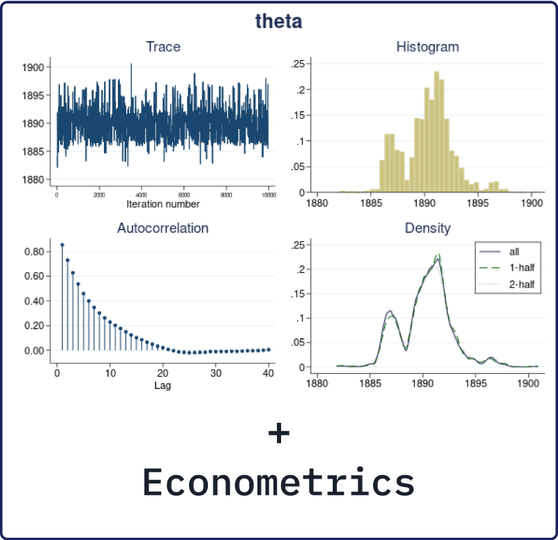
Bayesian econometrics
Stata 17 now does Bayesian econometrics. If you want to use probabilistic statements to answer economic questions, for example: “Are those who participate in a job-training program more likely to stay employed for the next five years?” or if you want to incorporate prior knowledge of an economic process then Stata’s new Bayesian econometrics features can help. Fit many Bayesian models such as cross-sectional; panel-data; multilevel; and time-series models. You can compare models using Bayes factors, obtain predictions and forecasts, and more!

PyStata—Python and Stata
Stata 17 introduces a concept called PyStata. PyStata is a term that encompasses all the ways Stata and Python can interact.
Stata 16 featured the ability to call Python code from Stata. Stata 17 greatly expands on this by allowing you to invoke Stata from a stand-alone Python environment via a new pystata Python package.
You can access Stata and Mata conveniently in an IPython kernel-based environment (for example, Jupyter Notebook and console; and Jupyter Lab and console); in other environments that support the IPython kernel (for example, Spyder IDE and PyCharm IDE); or when accessing Python from a command line (for example, Windows Command Prompt, macOS terminal, Unix terminal, and Python’s IDLE).

Jupyter Notebook with Stata
Jupyter Notebook is a powerful and easy-to-use web application that allows you to combine executable code, visualisations, mathematical equations and formulas, narrative text, and other rich media in a single document (a “notebook”) for interactive computing and developing. It is widely used by researchers and scientists to share their ideas and results for collaboration and innovation.
In Stata 17, as part of PyStata, you can invoke Stata and Mata from Jupyter Notebook with the IPython (interactive Python) kernel. This means you can combine the capabilities of both Python and Stata in a single environment to make your work easily reproducible and shareable with others.
The invocation of Stata from Jupyter Notebook is driven by the new pystata Python package.
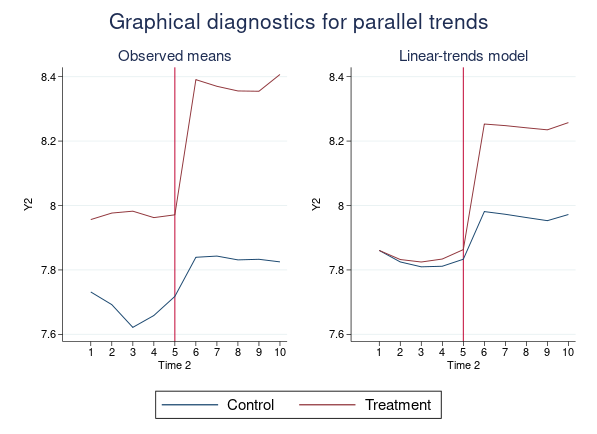
Difference-in-differences (DID) and DDD models
New estimation commands –didregress– and –xtdidregress– fit difference-in-differences (DID) and difference-in-difference-in-differences or triple-differences (DDD) models with repeated-measures data. –didregress– works with repeated-cross-sectional data, and –xtdidregress– works with longitudinal/panel data.
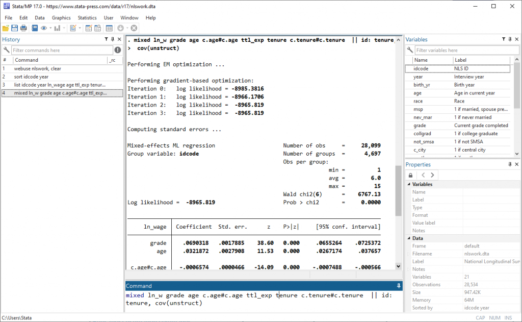
Making Stata faster
Stata values accuracy and it values speed. There is often a tradeoff between the two, but Stata strives to give users the best of both worlds. Stata 17 has updated algorithms behind sort and collapse to make these commands faster. Stata 17 incorporates speed improvements for some estimation commands such as mixed, which fits multilevel mixed-effects models.
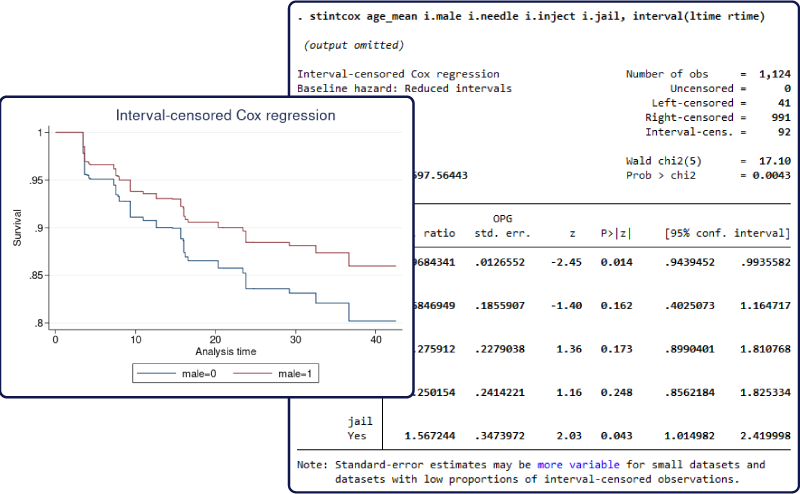
Interval-censored Cox model
A semiparametric Cox proportional hazards regression model is commonly used to analyse uncensored and right-censored event-time data. The new estimation command –stintcox– fits the Cox model to interval-censored event-time data.
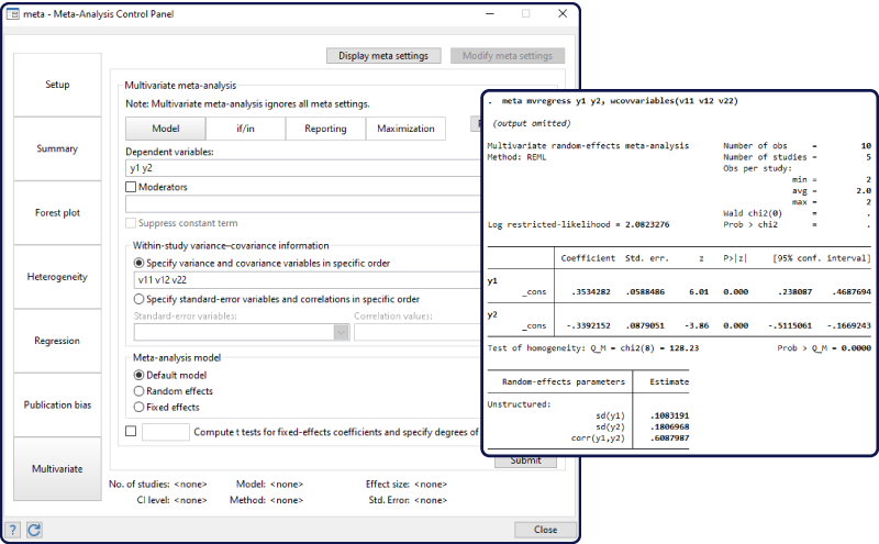
Multivariate meta-analysis
Use this new feature if you want to analyse results from multiple studies. The studies may report multiple effect sizes, which are likely to be correlated within a study. Separate meta-analyses, such as those using the existing meta command, will ignore the correlation. You can now use the new –meta mvregress– command to perform multivariate meta-analysis, which will account for the correlation.
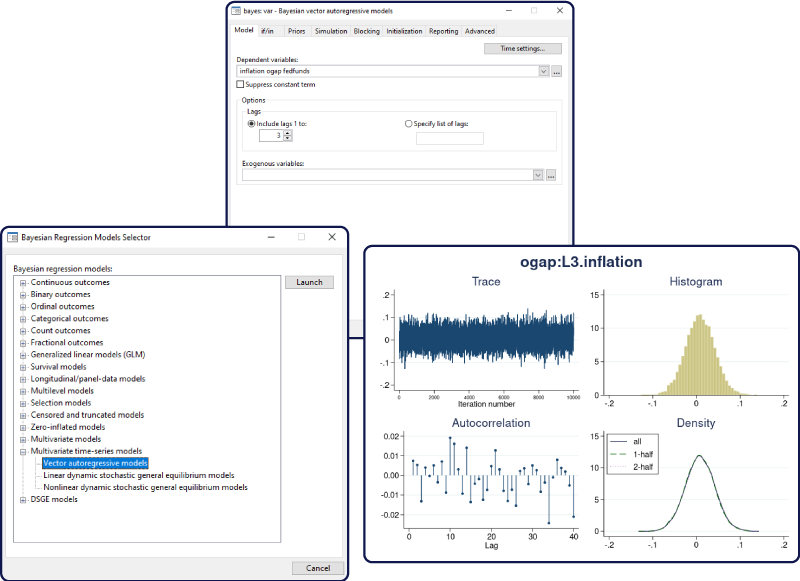
Bayesian VAR models
The bayes prefix now supports the –var– command to fit Bayesian vector autoregressive (VAR) models. VAR models study relationships between multiple time series by including lags of outcome variables as model predictors. These models are known to have many parameters: with K outcome variables and p lags, there are at least p(K^2+\nn1) parameters. Reliable estimation of the model parameters can be challenging, especially with small datasets. Bayesian VAR models overcome these challenges by incorporating prior information about model parameters to stabilise parameter estimation.
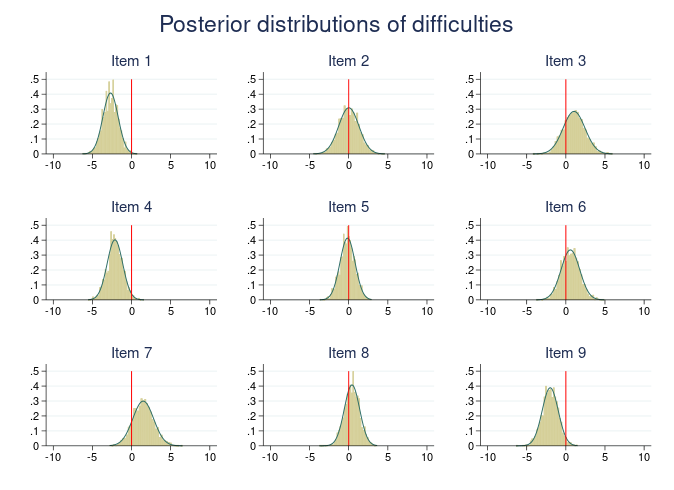
Bayesian multilevel modeling: Nonlinear, joint, SEM-like and more
You can fit breadth of Bayesian multilevel models with the new elegant random-effects syntax of the bayesmh command. You can fit univariate linear and nonlinear multilevel models more easily and you can now fit multivariate linear and nonlinear multilevel models! Think of growth linear and nonlinear multilevel models, joint longitudinal and survival-time models, SEM-type models, and more.
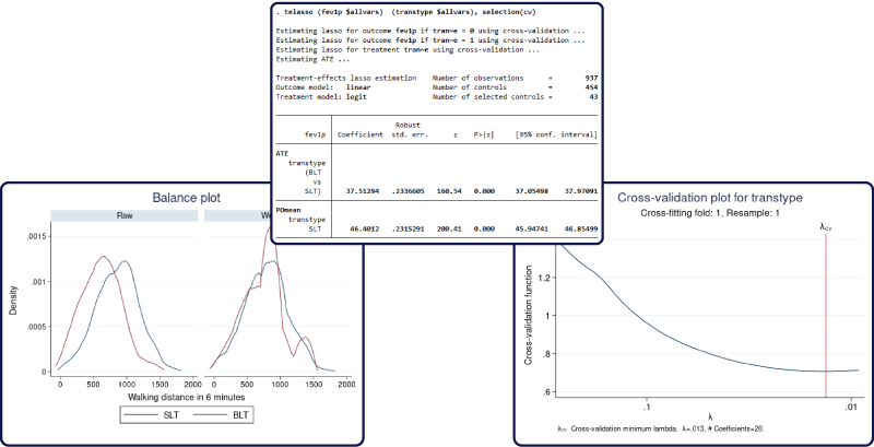
Treatment-effects estimation using lasso
You use –teffects– to estimate treatment effects. You use –lasso– to control for many covariates. And when we say many, we mean hundreds, thousands, or more! You can now use –telasso– to estimate treatment effects and control for many covariates.
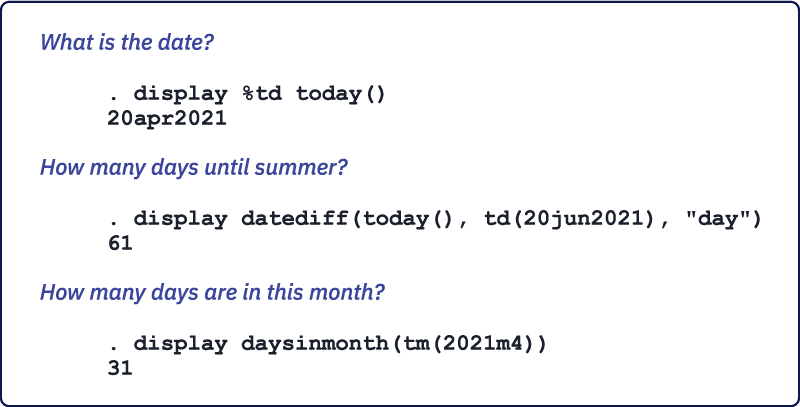
New functions for dates and times
Stata 17 has added new convenience functions for handling dates and times in both Stata and Mata. The new functions can be grouped into three categories:
- Datetime durations: functions that are designed to get durations, such as ages.
- Relative dates: functions that return dates based on other dates, such as the next birthday relative to a given date.
- Datetime components: functions that extract different components from datetime values.
The new functions factor in leap years, leap days, and leap seconds, wherever applicable. Leap seconds are one-second adjustments that are occasionally applied to Coordinated Universal Time (UTC).
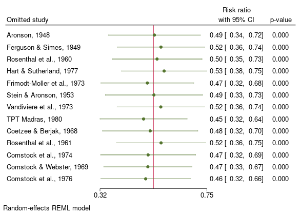
Leave-one-out meta-analysis
You can now perform leave-one-out meta-analysis by using the new option leaveoneout with –meta summarise– and –meta forestplot-. The leave-one-out meta-analysis performs multiple meta-analyses by excluding one study at each analysis. It is common for studies to produce exaggerated effect sizes, which may distort the overall results. The leave-one-out meta-analysis is useful to investigate the influence of each study on the overall effect-size estimate and to identify influential studies.
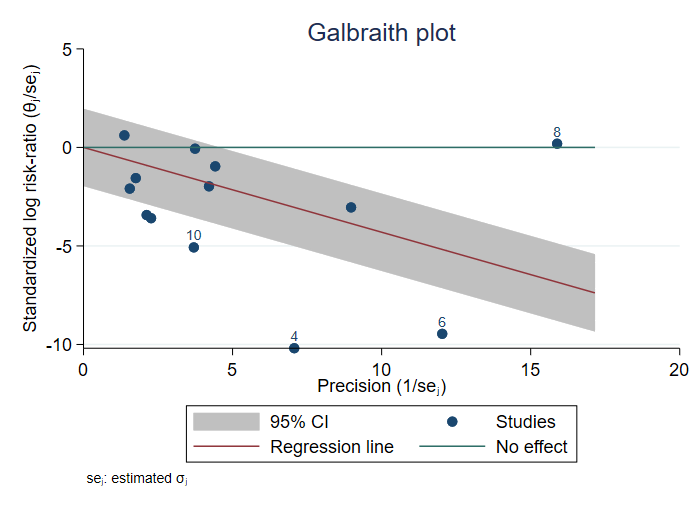
Galbraith plots
The new command –meta galbraithplot– produces Galbraith plots for a meta-analysis. These plots are useful for assessing heterogeneity of the studies and for detecting potential outliers. They are also used as an alternative to forest plots for summarising meta-analysis results when there are many studies.
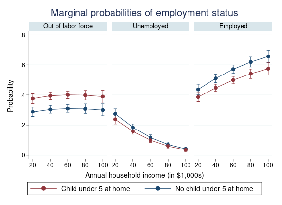
Panel-data multinomial logit model
Stata’s new estimation command –xtmlogit– fits panel-data multinomial logit (MNL) models to categorical outcomes observed over time. Suppose that we have data on choices of restaurants from individuals collected over several weeks. Restaurant choices are categorical outcomes that have no natural ordering, so we could use the existing mlogit command (with cluster–robust standard errors). But –xtmlogit– models individual characteristics directly and thus may produce more efficient results. And it can properly account for characteristics that might be correlated with covariates.
Bayesian longitudinal / panel-data models
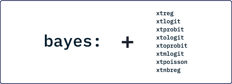
You fit random-effects panel-data or longitudinal models by using –xtreg– for continuous outcomes, –xtlogit– or –xtprobit– for binary outcomes, –xtologit– or –xtoprobit– for ordinal outcomes, and more. In Stata 17, you can fit Bayesian versions of these models by simply prefixing them with bayes.
Zero-inflated ordered logit model
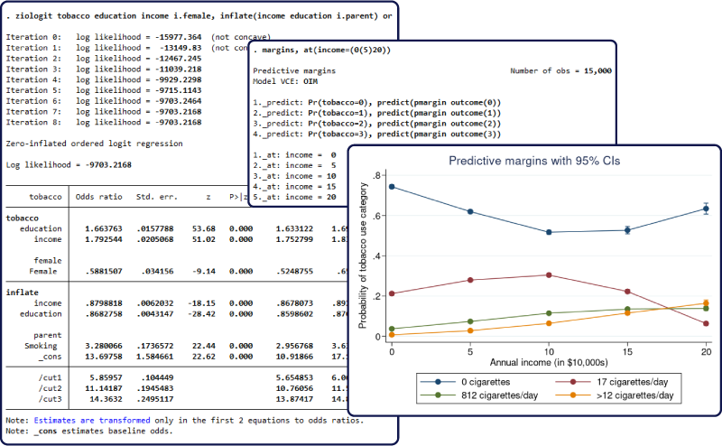
The new estimation command –ziologit– fits zero-inflated ordered logistic regression models. This model is used when data exhibit a higher fraction of observations in the lowest category than would be expected from a standard ordered logistic model. We refer to observations in the lowest category as zeros because they typically correspond to the absence of a behavior or trait. Zero inflation is accounted for by assuming that the zeros come from both a logistic model and an ordered logistic model. Each model can have different covariates, and the results can be displayed as odds ratios instead of the default coefficients.
Nonparametric tests for trend
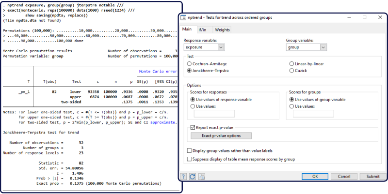
The –nptrend– command now supports four tests for trend across ordered groups. You can choose between the Cochran–Armitage test, the Jonckheere–Terpstra test, the linear-by-linear trend test, and the Cuzick test using ranks. The first three tests are new, and the fourth test was performed by nptrend previously.
Bayesian IRF and FEVD analysis
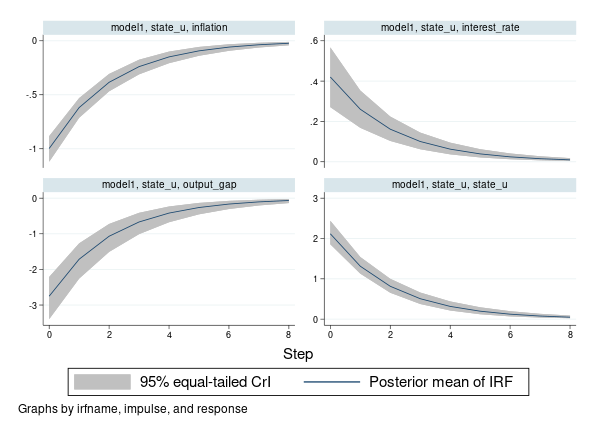
Impulse–response functions (IRFs), dynamic-multiplier functions, and forecast-error variance decompositions (FEVDs) are commonly used to describe the results from multivariate time-series models such as VAR models. VAR models have many parameters, which may be difficult to interpret. IRFs and other functions combine the effect of multiple parameters into one summary (per time period). For instance, IRFs measure the effect of a shock (change) in one variable on a given outcome variable.
Bayesian IRFs (and other functions) produce the results using the “exact” posterior distribution of IRFs, which does not rely on the assumption of asymptotic normality. They may also provide more stable estimates for small datasets because they incorporate prior information about the model parameters.
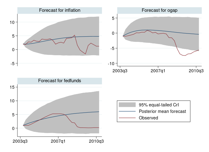
Bayesian dynamic forecasting
Dynamic forecasting is a common prediction tool after fitting multivariate time-series models, such as vector autoregressive (VAR) models. You use –fcast– to compute dynamic forecasts after fitting a classical var model. You can now use –bayesfcast– to compute Bayesian dynamic forecasts after fitting a Bayesian VAR model using bayes: var.
Bayesian dynamic forecasts produce an entire sample of predicted values instead of a single prediction as in classical analysis. This sample can be used to answer various modelling questions, such as how well the model predicts future observations without making the asymptotic normality assumption when estimating forecast uncertainty. This is particularly appealing for small datasets for which the asymptotic normality assumption may be suspect.
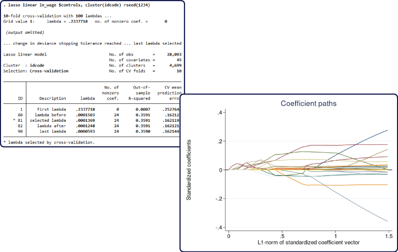
Lasso for clustered data
You can now account for clustered data in your lasso analysis. Ignoring clustering may lead to incorrect results in the presence of correlation between observations within the same cluster. With lasso commands for prediction such as –lasso– and –elasticnet-, you can specify the new cluster ({\it clustvar}) option. With lasso commands for inference such as poregress, you can specify the new –vce(cluster {\it clustvar})– option.
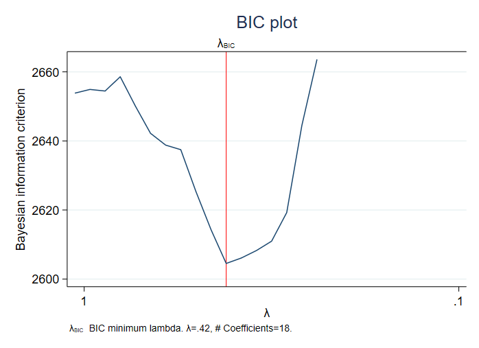
BIC for lasso penalty selection
Selection of a penalty parameter is fundamental to lasso analysis. Using a small penalty may include too many variables. Using a large penalty may omit potentially important variables. Lasso estimation already provides several penalty-selection methods, including cross-validation, adaptive, and plugin. You can now use the Bayesian information criterion (BIC) to select the penalty parameter after lasso for prediction and lasso for inference by specifying the selection(bic) option. Also, the new postestimation command bicplot plots the BIC values as a function of a penalty parameter after fitting a lasso model. This provides a convenient graphical representation for the value of the penalty parameter that minimises the BIC function.
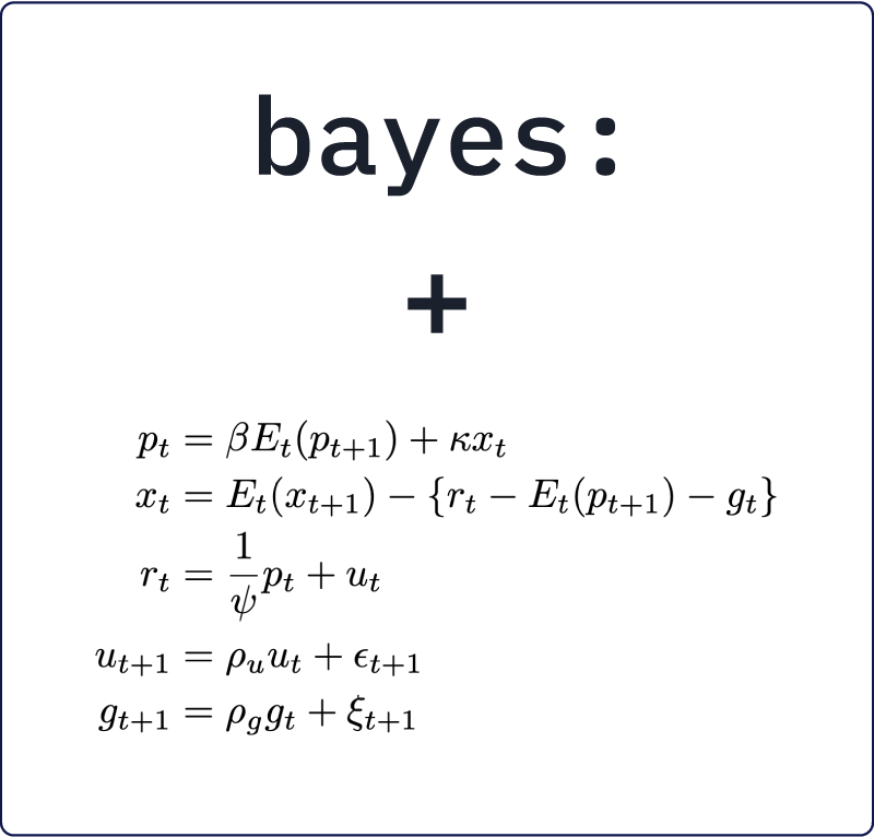
Bayesian linear and nonlinear DSGE models
You can now fit Bayesian linear and nonlinear dynamic stochastic general equilibrium (DSGE) models by prefixing –dsge– and –dsgenl– with –bayes:-. Incorporate information about the ranges of model parameters by choosing from over 30 different prior distributions. Perform Bayesian IRF analysis, perform interval hypothesis testing, use Bayes factors to compare models, and more.

Do-file Editor improvements: Bookmarks
Bookmarks are used to mark lines of interest to navigate to them later more easily. Bookmarks are particularly useful in navigating long do-files. You can add bookmarks to sections of your do-files that perform data management, display summary statistics, and perform statistical analysis. You can then use the menus, the toolbar, or the new Navigation Control to quickly move back and forth between those sections without having to scroll through several lines of code to find the section that you are looking for.

Do-file Editor improvements: Navigation control
Stata 17 makes navigating do-files easier with the new Navigation Control, which displays a list of bookmarks and their labels. Selecting a bookmark from the Navigation Control will move the Do-file Editor to the bookmark’s line. In addition to bookmarks, the Navigation Control will also display a list of programs within a do-file. Selecting a program from the Navigation Control will move the Do-file Editor to the program’s definition. No extra effort is needed to add a program to the Navigation Control. The Do-file Editor will automatically add a program’s definition to the Navigation Control.
Stata on Apple Silicon
Stata 17 for Mac is available as a universal application that will run natively on both Macs with Apple Silicon and Macs with Intel processors. Macs with Apple Silicon include the new MacBook Air, MacBook Pro, and Mac mini, all with M1 processors. The M1 chip promises greater performance and greater power efficiency. This is noteworthy to our Stata-for-Mac users, many of whom use Mac laptops.
Although this first set of M1 Macs is considered to be an entry-level set, we have found that M1 Macs natively running Stata outperform Intel Macs by 30–35%. They even greatly outperform or perform as well as Intel Macs that cost more than twice as much! And for users who insist on only Apple-Silicon-native software on their Apple Silicon Macs, you will be happy to know that no part of Stata 17, from the installer to the application itself, requires the use of Rosetta 2.
Stata functions the same way whether you are running Stata natively on an M1 Mac or on an Intel Mac, and no special licence is required for the M1 Mac. Intel Mac users should note that we will continue to support and release new versions of Stata for Macs with Intel processors for years to come.
Intel Math Kernel Library (MKL)
Stata 17 introduces usage of the Intel Math Kernel Library (MKL) on compatible hardware (all Intel- and AMD-based 64-bit computers), providing deeply optimised LAPACK routines.
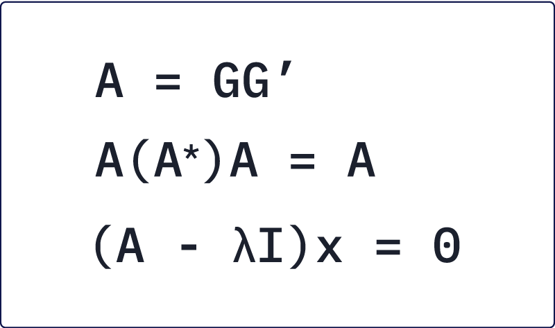
LAPACK stands for Linear Algebra PACKage and is a freely available set of routines for solving systems of simultaneous equations, eigenvalue problems, and singular-value problems, among others.
Mata operators and functions (such as qrd(), lud(), and cholesky()) leverage LAPACK where possible for many numerical operations.
LAPACK backed by the Intel MKL provides the latest LAPACK routines heavily optimised for the 64-bit Intel x86-64 instruction set used by both modern Intel and modern AMD processors. Mata functions and operators using MKL benefit greatly in terms of performance.
And most importantly, you do not need to do anything to take advantage of the speed gains. Stata commands using these Mata functions and operators, and the Mata functions and operators themselves, will automatically use the Intel MKL on compatible hardware.

Java integration
In Stata 17, you can now embed and execute Java code directly in Stata. You could already create and use Java plugins in previous versions of Stata, but that required you to compile your code and bundle it in a Jar file. Executing Java in a do-file gives you the freedom to execute Java code tied directly to your Stata code. Now you can write your Java code in do-files or ado-files, or even invoke Java interactively (like JShell) from within Stata.
One of Java’s strengths is in its extensive APIs that are packaged with the Java virtual machine. There are also many useful third-party libraries available. Depending on what you need to do, you may even be able to write parallelised code to take advantage of multiple cores.
The Java code you write compiles on the fly. There is no need to use an external compiler! Additionally, the Stata Function Interface (SFI) Java package is included, providing a bidirectional connection between Stata and Java. The SFI package has classes to access Stata’s current dataset, frames, macros, scalars, matrices, value labels, characteristics, global Mata matrices, date and time values, and more.
Stata bundles the Java Development Kit (JDK) with its installation, so there is no additional setup involved.

H2O integration
In Stata 17, you can experiment with connecting to H2O, a scalable and distributed open-source machine-learning and predictive analytics platform. Read more about H2O at https://docs.h2o.ai/.
With the integration of H2O, you can start, connect to, and query an H2O cluster from Stata. In addition, we provide a suite of commands to manipulate data (H2O frames) on the cluster. For example, you can create new H2O frames by importing data files or loading Stata’s current dataset. You can also split, combine, and query H2O frames from within Stata.
Although this is still in the experimental stage, StataCorp want to make it available to Stata users to try it out. On the other hand, because it is an experimental feature, syntax and features are subject to change. When using Stata commands that provide access to a given feature of H2O, keep in mind that that is an H2O feature. While you may be accessing H2O via a Stata command, what H2O does is up to H2O and is outside of Stata.

JDBC
Connecting Stata with databases is now even easier. Stata 17 adds support for JDBC (Java Database Connectivity). JDBC is a cross-platform standard for exchanging data between programs and databases.
The new –jdbc– command supports the JDBC standard for exchanging data with relational databases or nonrelational database-management systems that have rectangular data. You can import data from some of the most popular database vendors, such as Oracle, MySQL, Amazon Redshift, Snowflake, Microsoft SQL Server, and many more. What is great about –jdbc– is that it is a cross-platform solution, so our JDBC setup works the same way for Windows, Mac, and Unix systems.
If your database vendor provides a JDBC driver, you can download and install that driver and then read from, write to, and execute SQL on your database via jdbc. You can load an entire database table into Stata or use SQL SELECT to just load specific columns from a table into Stata. You can also insert all your variables into a database table or just insert a subset of your dataset.
